sidmon is a python program for receiving and recording submarine-transmitter signal intensities in the VLF frequency range using a computer sound card and the alsaaudio package. The intensities of these signals reflect the ability of radio waves at those wavelengths to propagate in what is essentially a waveguide formed by the earth and the ionosphere above it. Fluctuations in those signal intensities often reflect daytime perturbations of the ionosphere by solar processes, such as solar flares and coronal mass ejections, making VLF receivers useful tools for probing the sun and the earth's ionosphere. For more information see the SID Monitors page and the SID data access page at the Stanford Solar Center.
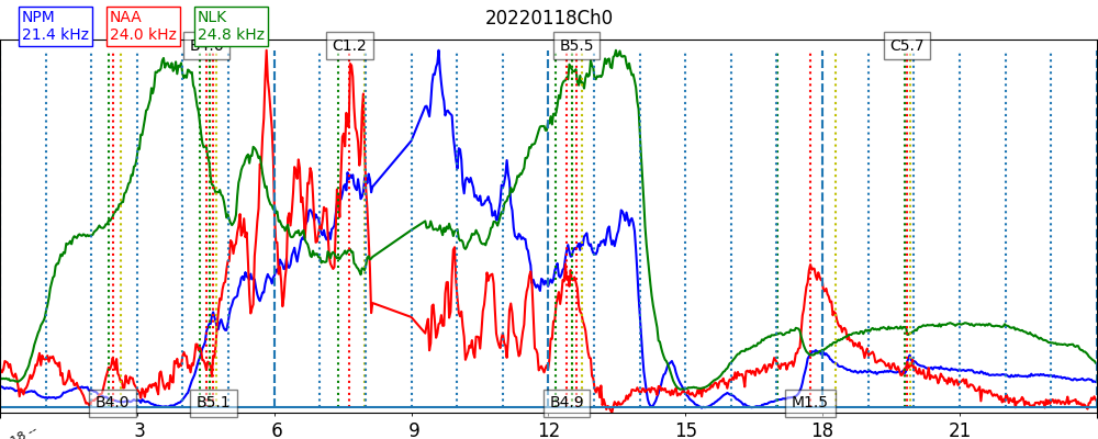
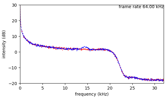
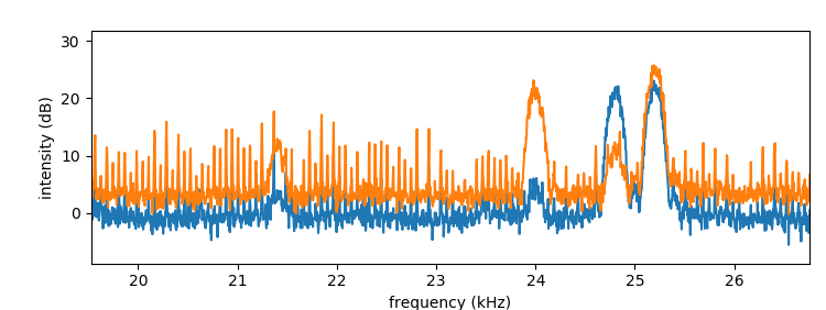
sidmon can record multiple stations simultaneously. In my tests, there is no amplification of the antenna signal or other signal conditioning. Antenna tuning can be employed but is not necessary. See the equipment section below for a description of my setup. The first graph is an example of the system's performance, showing two SIDs on three transmitter traces.
A feature of the code is that it estimates the frequency-dependent background level so that it can be separated from line intensities. Noise typically varies, and a good estimate of it reduces scatter to allow detections of smaller SIDs.
Once transmitter intensities are measured by sidmon they are output to a file with a header more or less like the Stanford SID file headers. More than one transmitter may be recorded to this file.
There is a live-plot feature that plots spectra in real time, allowing visualization and identification of transmitter lines. Two other features are antenna tuning, and transient excision. Setup and use of these two features are not given here; but they are not necessary to get started, and often are not needed at all.
A guide to setup of a Raspberry Pi and installation of sidmon are given in a companion document. But note that the computer need not be a Raspberry Pi, such as a laptop or desktop.
Run the program from its directory giving the sound-device name with the -d switch.
./sidmon.py -d <device> -lp 1
where <device> is the sound-card device identified with the arecord -L command (see the installation guide). A graph of the spectrum of the antenna input (with the -lp 1 switch) is updated each cycle. To exit the program enter control+c
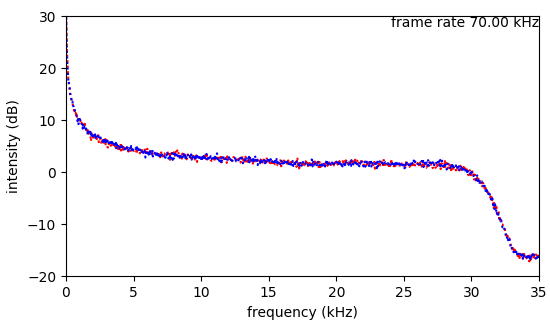
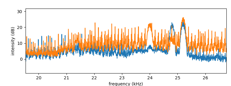
An example spectrum is shown in the next graph. The sample rate is 64 kHz where the first Nyquist zone up to 32 kHz is shown. There is no antenna tuning, which is how I suggest new users start.
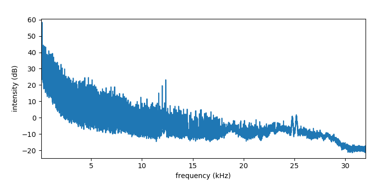
Lines corresponding to two transmitters, at 24.8 and 25.5 kHz (NLK and NML), are visible in the graph. There is a lot of noise present in the spectrum, much of it being power-line harmonics.
There is a third transmitter visible at 21.4 kHz (NML). Although buried in the noise, the outlier feature of the fitting process (next section) can nicely dig the intensity out of the noise. In addition, NAA at 24.0 kHz is often strong at my location, and I also monitor NWC in Australia at 19.8 kHz for the fun of it, for a total of five transmitters.
As illustrated by this example, live-plot 1 is the tool to use to determine monitorable transmitters at a given location.
To change the monitored transmitters, modify the file Header.txt to reflect the new transmitters. When a new data file is created at the start of a new UTC day, the new file will reflect the transmitter choices contained in the revised Header.txt file.
Fitting is used to measure line intensities. The basis functions consist of a low-order polynomial for the background, and a line shape function that is typically Gaussian. In principle the widths can be different for the different transmitters, but in practice the widths are the same among them. One may choose alternate line shapes as needed. At my location, for example, NML has sufficient strength that a number of sidelobes are visible; Interestingly, the line shape of this transmitter is accurately modeled by a combination of sine integrals times an even, second-degree polynomial. Use of more complex line models can improve the fits, although perhaps with diminishing returns.
Lines/transmitters are divided into groups with members in close proximity, each group having a common polynomial basis and lines in the group fitted together with the basis. The next figure is the result of a fit four groups, having one, one, one, and two members, respectively. The frequency span of a group is chosen to contain the lines with margins for additional background. In those graphs, the blue trace is the raw data, the red trace the fit, and the green trace is the residual. In practice, one adjusts the polynomial and line basis functions to minimize the residual, such as by adjusting the width and center frequency of a line.
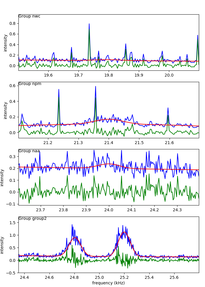
In this example, the first and third groups show no measureable line intensities, while the second shows a marginal – but real – intensity, and the fourth group measures two strong lines.
Note in the second group the presence of strong and narrow lines at harmonics of the line frequency. It is an important feature of sidmon that during the fitting process, these lines are recognized as outliers and excluded from the intensity points fitted to the basis. This way, these lines, even though intense, do not contaminate the fitted line intensities, resulting in more accurate measured intensities, particularly for weak lines. It is able to do this because these noise lines are sparse. For a given sample count in a Fourier frame, a lower sample rate spreads those lines between more Fourier (spectral) bins, increasing sparsity. For this reason it is helpful to use a lower sample rate when the observed transmitters can still be contained in the first Nyquist zone (sample rate / 2).
An example header file is this
# Site = <site id assigned by Rodney Howe>
# Contact = <contact information>
# Longitude = <longitude decimal degrees>
# Latitude = <latitude decimal degrees>
# Elevation = <elevation meters (not required)>
# LogInterval = 4.87
#
# Stations = NPM, NAA, NPMd, NAAd
# Frequencies = 21400, 24000, 21400, 24000
#
# supersid_plot parameters above here
# ###################################
# sidmon parameters below here
#
# antenna card: name, gain, angle
# antenna = ant0, 0.89, 166.0
#
# sound-card frame rate in Hz
# sampleratesetting = 68400
# sampleratemeasured = 68400.0
#
# number of frames in fourier frame (no need to change)
# fourierframe = 16384
#
# requested integration time (same as LogInterval above)
# integrationtime = 4.87
#
# sound channel count (1 or 2 (stereo); 1 disables 2nd antenna and direction capability)
# channelcount = 1
#
# group = npm, 21100, 21700, 1
# transmitter = NPM, 21400, lambda f: np.exp(-((f - 21400)/47)**2/2), -71.4, +21.420166, -158.151140, Pearl Harbour; Lualuahei; HI
#
# group = naa, 23600, 24400, 1
# transmitter = NAA, 24000, lambda f: np.exp(-((f - 24000)/47)**2/2), 85.2, +44.644936, -067.281639, Cutler; ME
The header file tells sidmon about the transmitters, how to perform line fitting, and other information inherited from SuperSID. Each line starts with the comment (#) character.
The transmitter names and frequencies are given in the Stations and Frequencies lines. These are used by supersid_plot.py to annotate the graphs to identify traces. sidmon does not use the information.
The antenna, fourierframe, integrationtime, and channelcount lines are used by sidmon. The remainder of the lines are for the fitter specifying one or more groups containing one or more transmitters. Each group consists of a group line followed by transmitter lines.
A group line has the form
# group = <name>, <freqlow>, <freqhigh>, <order>where
A transmitter line can contain a number of symbolic parameters given in name, value pairs. The entire line has the form
# transmitter = <name>, <freqnom>, <k>, <param1>, <val1>, ..., <paramk>, <valk>, <function>where
The example above contains two groups consisting of one transmitter, and one group consisting of two transmitters. Each transmitter line contains the parameters f0 that represents the actual transmitter frequency used in the fitting, and can differ from the nominal. The parameter sig is used to parameterize the width of the line. The last transmitter parameter, the function, is given as a python lambda expression.
The transmitter names and frequencies in the groups definitions should be the same as in the Stations and Frequencies lines. Yes, there is redundance.
The header file is read when sidmon starts. When a new file is created, such as as at the start of a new day, the contents of the header file becomes the header of the data file. When sidmon> is started when there is an existing data file for that data, the existing header is not changed, but the header file contents determines the how data are taken subsequently. Same with changed switches such as the veto threshold (next section). This means that, for example, when a transmitter is added to the header file and sidmon restarted, the number of columns in the data changes and plotting will fail for this reason. So when possible, allow the new header file to take effect at the start of a new day when a new fil is automatically created.
Important requirements of the sound card are
Specifications available for consumer sound cards typically do not provide these figures. So sound cards not otherwise known to work with sidmon need to be tested. Before trying to run sidmon it is important that the various sound-card frame rates be tested to show that they 1) work at all (do not generate obscure errors), and 2) that the one chosen meets the requirements above.
The program audio.py is available for basic tests of the audio card and the audio environment. To list the installed sound cards,
$ src/audio.py cards
HDMI
PCH
To list available sound devices,
$ src/audio.py devices
...
plughw:CARD=PCH,DEV=0
usbstream:CARD=PCH
sysdefault:CARD=Device
front:CARD=Device,DEV=0
...
Of course, other tools, such as arecord -L, are available for these functions. To plot the spectrum of a sound device, use
$ src/audio.py spectrum <device> <framerateHz> [<updateintervalsec>]So entering
src/audio.py spectrum plughw:CARD=Device 64000on my system results in
This graph (without an antenna) shows, first that it is acquiring at the selected frame rate; second is the analog bandwidth, the frequency at which the level drops off; and third that there are two distinct analog channels (red and blue points) available. In this case the bandwidth is 22 kHz, inadequate for monitoring, for example, NML at 25.2 kHz. At a higher frame rate the bandwidth is over 30 kHz.
src/audio.py spectrum plughw:CARD=Device 70000
Finally, be sure that the two audio input channels are actually connected to the input connector by connecting two antennas to the audio input. Both traces should show much stronger signals.
The last function measures the sound card's frame rate accurately, which is needed to determine a frame rate that meets requirement 3 above. Perhaps the frame rate of most sound cards can be set sufficiently accurately with a harmonic setting. But this is not always the case, and a measurement of the frame tells us whether it is. Use the syntax
# src/audio.py measurerate <device> <framerate> <durationmin> <printintervalsec>
src/audio.py measurerate plughw:CARD=Device 64000 10 30
{
  {29.986239,1919190,64002.35788,1365},
  {59.974466,3838380,64000.23637,1365},
  {89.960897,5757570,64000.80693,1365},
  {119.947453,7676760,64001.02552,1365},
  {149.934907,9595950,64000.77335,1365},
  ...
It will periodically print out a frame rate averaged over the duration of the acquisition. The cumulative rate is in the third column. Exit using control c. With knowledge of the exact frame rate at one setting, compute the setting for the target frame rate.
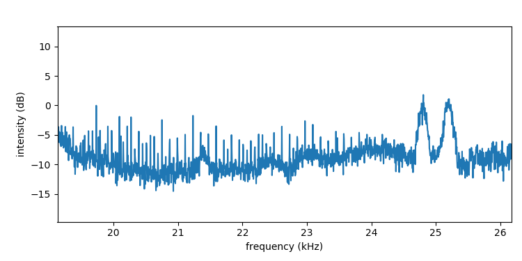
Sound-card gain settings can also be optimized using audio.py while changing settings using alsamixer. Do this with an antenna connected to the sound card. Using the spectrum feature, enter
src/audio.py spectrum <device> <framerate>One or more of the transmitter lines to be monitoried must be visible. In this example NLK and NML are present at 24.8 and 25.2 kHz.
Zoom in on the lines using the figure's zoom button. The signal-to-noise ratio (S/N) in dB is the difference between the peak height and the background level, which is about 10 dB in this case. The task is to maximize that ratio using gain settings controlled by alsamixer running in another terminal. At some point when the gain is increased, the background noise level will continue increasing while the line intensities slow or stop increasing, indicating a falling S/N. Going the other way with decreasing gain, at some point the background level will slow or stop falling while the line intensity continues falling – again indicating falling S/N. In this way a range of gain settings with good S/N is identified, and settings toward the lower end of that range are chosen.
Another noise-reduction feature is the 'veto' feature. This is a more advance feature, and I suggest also skipping setup of this feature when first getting your receiver running.
This feature looks for and excludes blocks in the data stream with excess noise. Excess noise can happen when an electrical glitch injects noise into the data stream, such as when there is lightning in the viscinity. We classify these as transient noise events. Even if they are infrequent, they can still degrade the receiver performance because they are often intense. This is why excluding these noisy blocks can clean up the spectra significantly.
To use this feature, a noise threshold for the exclusion must be set. sidmon is always accumulating a histogram of these block intensities, and when the program is exited after it has been running for a while, this histogram is appended to the file <machinename>.hist. Plot it with hist.py.
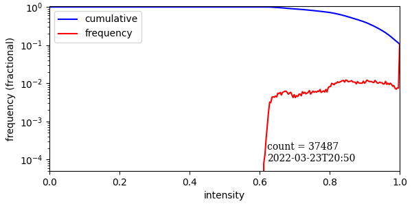
src/hist.py --prev -1where the data are taken from <machinename>.hist. The index -1 specifies the most recent histogram; specify an earlier histogram with a more negative index. The following is an example.
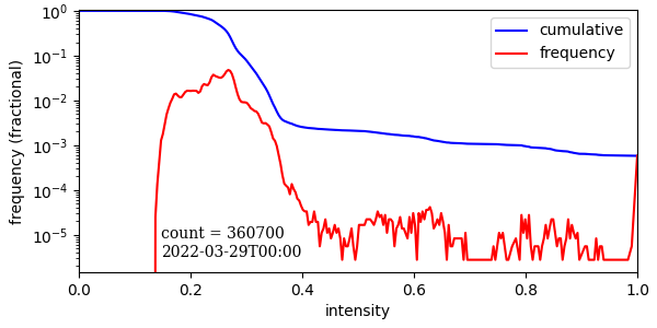
The red trace is the fractional part of the of Fourier Frames at which that intensity occurs. The blue trace is the fraction of Fourier frames whose intensity are above that intensity. Choose a threshold that admits almost all the numerous 'normal' points at lower intensities, but excludes the much-less-frequent higher-value outliers. In the example of the plot above, one might choose the break in the red trace at 0.45.
Then rerun sidmon with the -v (--veto) switch:
src/sidmon.py -d plughw:U5 --veto 0.8
The next question is 'How do I know it is working?'. The lines printed in either the command window, or a file to which stdout is redirected, will periodically print the accumulated rejected Fourier frames. A few lines of that output stream:
2022-01-20 13:49:44.38, sumcrt 19, matrix errors 0, overruns 0, vetos 305
2022-01-20 13:51:41.63, sumcrt 19, matrix errors 0, overruns 0, vetos 307
2022-01-20 13:53:38.88, sumcrt 19, matrix errors 0, overruns 0, vetos 309
2022-01-20 13:55:36.14, sumcrt 19, matrix errors 0, overruns 0, vetos 311
2022-01-20 13:57:33.14, sumcrt 19, matrix errors 0, overruns 0, vetos 312
2022-01-20 13:59:29.87, sumcrt 19, matrix errors 0, overruns 0, vetos 312
Each line consists of a date and time, followed other parameters, and finally by a cumulative veto count of excluded frames. If that count stays at zero, then either there are no glitches (maybe), or the threshold is too high. Alternatively, if the count accumulates very rapidly, it is likely that the threshold is too low and should be raised. I would suggest that you set the threshold so that the count accumulates rather slowly and experiment from there.
The final say about this feature's effectiveness is in the number of glitches that are evident in the day's plot of receiver intensities. There can be many such glitches depending on the severity of the RFI environment. Experiment with the threshold from day to day and see if the quality of your data imporoves.
src/sidmon.py [options ...]
Options.
Stop sidmon using these methods:
$ touch quitfrom another terminal in the running-program's current directory.
kill -s 2 <processid>where the process id of the process is given.
An example command line where the program is run from the sidmon root directory is this.
src/sidmon.py -d plughw:CARD=MKII,DEV=0 -t 4.5 -lp 1 --header exampleheader.txt
To run in the background,
nohup src/sidmon.py -d plughw:CARD=MKII,DEV=0 -t 4.5 -s 88200 &
src/supersid_plot.py [options ...]
Options
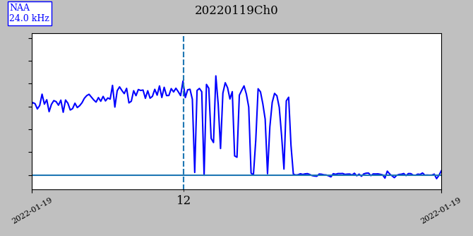
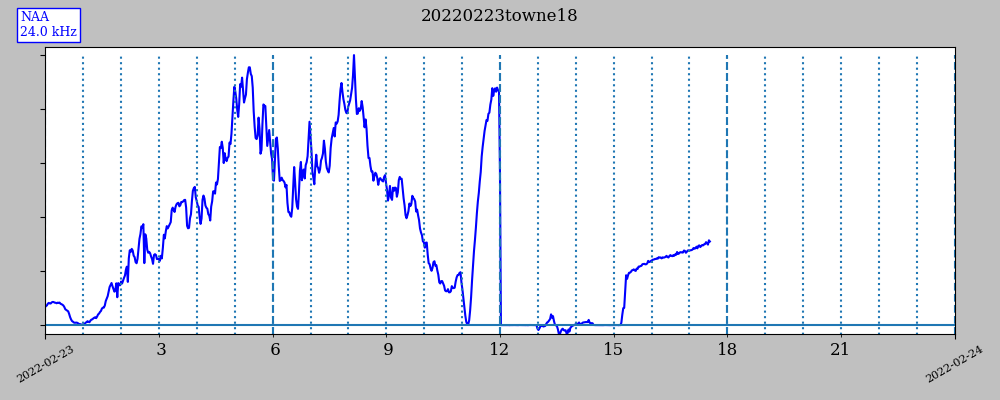
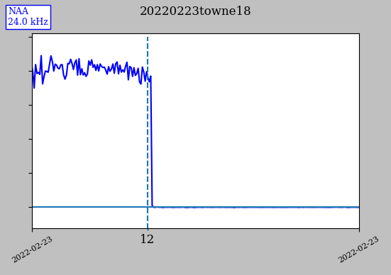
To illustrate decimation, the following graph with decimation = 1 (no decimation) shows NAA shutting down at noon UT. It is curious that it took four ratty minutes to do so.
src/supersid_plot.py -f data/20220119Ch0.csv --decim 1
Noise in the environment is inevitable, and it impacts sidmon results. My results have been very good, but from feedback from others using sidmon, results are not always so good. It is helpful to users to be aware of this reality, and how noise problems can be diagnosed.
The most important tool for close looks at data is the live-plot feature mentioned in the options section. This feature displays raw spectra of the one or two sound channels being captured from the sound card. An example is the second figure of this document. Most commonly there are fluctuations of the spectrum that varies the level, slope, and curvature of the spectrum in the viscinity of a transmitter line. Although not particularly good examples, the following three spectra illustrate how this can happen. The first is relatively quiet spectrum.
Followed by a spectrum with a fluctuation near the NAA line at 24.0 kHz, capable of affecting the noise measurement moderately.

The disturbance responsible for this fluctuation may be intense enough that the veto feature may be effective against it, although they are likely too dense for the outlier feature to work.
These fluctuations can at times wreak havoc on the intensity-measurement methods employed by sidmon. An older intensity graph shows a periodic disturbance.
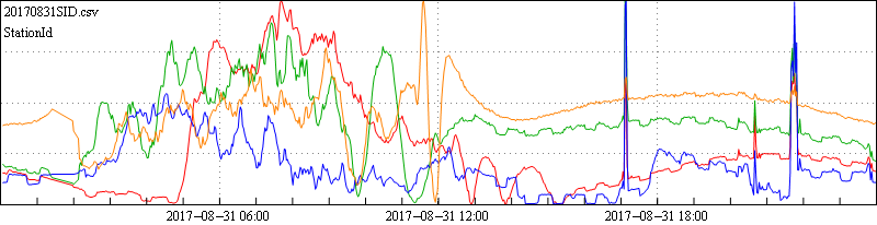
In a more recent example, a noise source switched on and later off during a time the transmitter was shut down. The transmitter shut off at 1200 UT and on at 1520 UT.
To see clearly the shutoff and the precision of the zero-power measurement, we zoom in while setting the decimation to 1 for the full five-second resolution of the data set.
The power is seen to drop to zero with very high contrast. Zooming out again to cover the entire time the transmitter was off, we see this.
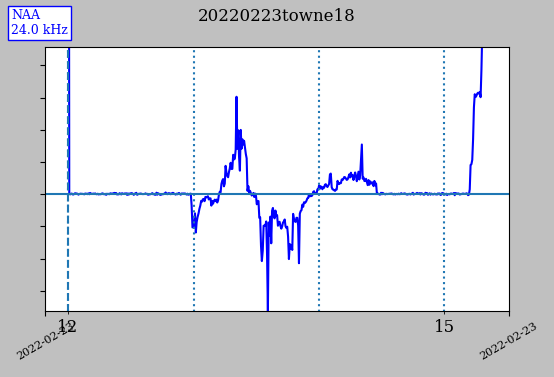
In the middle of the interval, there is a 1.5 hour period during which a noise source switched on, generating fluctuations in the measured signal intensity that goes both positive and negative by a degree much greater than the relatively noise-free fluctuations before and after. The following histogram shows intensities during a period in which a noise source was on.
With the veto feature active during this period, no data are taken before the veto limit is reached (--vetoclim <limit>). This limit is needed for when a noise source remains active for minutes, hours, or days, during which time no data would otherwise be taken. The rationale is that is is better to have noisy data during such long intervals than none at all.
Nathan Towne
towne56 at ownmail dot net
1/2022
Comments and bug reports are welcome.