sidmon 2 is a python program for receiving and recording submarine-transmitter signal intensities in the VLF frequency range using a computer sound card and the alsaaudio package. The intensities of these signals reflect the ability of radio waves at those wavelengths to propagate in what is essentially a waveguide formed by the earth and the ionosphere above it. Fluctuations in those signal intensities often reflect daytime perturbations of the ionosphere by solar processes, such as solar flares and coronal mass ejections, making VLF receivers useful tools for probing the sun and the earth's ionosphere. For more information see the SID Monitors page and the SID data access page at the Stanford Solar Center.
sidmon 3 is an enhanced sidmon 2 that can employ two loop antennas that are combined to form a simple phased array. With a single loop, the signal intensity of a transmitter depends on the orientation of the loop relative to the great arc to the transmitter. A loop is most sensitive if it is edge on (tangent) to the great arc, while an orthogonal loop intercepts no magnetic flux and hence has zero sensitivity to that transmitter. Two loops, in contrast, can be combined with weights that 'point' the combined loops toward a transmitter, catching maximum flux into the data stream, while injecting equivalent noise of only one ADC. This can be done digitally for each transmitter being monitored. In this sense, the antenna/receiver system become isotropic - able to receive with equal sensitivity in all directions.
sidmon 3 synthesizes the beam orthogonal to the transmitter along with the one pointing to the transmitter. Although that orthogonal beam intercepts no flux from signals on its pointing, it is sensitive to deviations from its pointing, such as when there are deflections of the beam by tilts of the ionospheric electron density. So the orthogonal beam, in conjunction with the main beam, can measure signal direction, and detect direction transients associated with SIDs. In fact, there is remarkable sensitivity realized in sidmon 3 of typically < 0.1 degree (on one-minute integrations for stronger signal), that provides another way to detect SIDs and how the ionosphere is impacted by x-rays from solar flares.
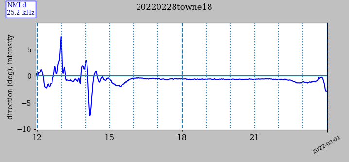
In the following figure, the uncalibrated intensity is the blue trace, while the calibrated direction relative to the primary beam pointing is the red trace, to which the vertical scale applies. There is a SID detection after 1900 UT, evident in both the intensity trace and direction trace.
The sidmon 2 usage document describes most of the setup of a sidmon 3 observatory. The remainder of this document describes the setup of the loop antennae and beam pointing specific to sidmon 3.
An example header file monitoring two transmitters in two goups and recording directions is this.
# Site = <site id assigned by Rodney Howe>
# Contact = <contact information>
# Longitude = <longitude decimal degrees>
# Latitude = <latitude decimal degrees>
# Elevation = <elevation meters (not required)>
# LogInterval = 4.87
#
# Stations = NPM, NAA, NPMd, NAAd
# Frequencies = 21400, 24000, 21400, 24000
#
# supersid_plot parameters above here
# ###################################
# sidmon parameters below here
#
# antenna card: name, gain, angle
# antenna = ant0, 0.89, 166.0
# antenna = ant1, 1.0, 76.0
# antrefl = False
#
# sound-card frame rate in Hz
# sampleratesetting = 68400
# sampleratemeasured = 68400.0
#
# number of sound frames in fourier frame (no need to change)
# fourierframe = 16384
#
# requested integration time (same as LogInterval above)
# integrationtime = 4.87
#
# sound channel count (1 or 2 (stereo); 1 disables 2nd antenna and direction capability)
# channelcount = 2
#
# group = npm, 21100, 21700, 1
# transmitter = NPM, 21400, lambda f: np.exp(-((f - 21400)/47)**2/2), -71.4, +21.420166, -158.151140, Pearl Harbour; Lualuahei; HI
#
# group = naa, 23600, 24400, 1
# transmitter = NAA, 24000, lambda f: np.exp(-((f - 24000)/47)**2/2), 85.2, +44.644936, -067.281639, Cutler; ME
Some of this is mentioned in the sidmon 2 usage document. When running in the dual-channel mode, there are additions in the Stations and Frequencies lines for the benefit of supersid_plot.py because sidmon outputs directions as well as intensities. The additional names are arbitrary, but must be distinct. There are also additional parameters in the transmitter lines.
The antenna lines are there to provide the gain parameter. In the example above, there is an additional parameter giving the antenna's orientation relative to geographic north, for reference. But it is not currently used by sidmon.
The parameters samplerate, fourierframe, channelcount, and integrationtime are present in the file and should not be given on the commandline. The sample rate is in Hz; the fourier frame sample count should not be changed; and the integration time is in seconds. The last is a duplicate of the LogInterval parameter.
The transmitter lines have one additional required parameter beyond those required by sidmon 2, which is the beam direction in degrees as determined by the scan plot. In the example above there are also latitude, longitude, and a description string placed there for reference.
To measure source direction, two loop antennae are required. It is preferable to fabricate them identically, although antenna gains in the header file can compensate for differences. For example, imagine two antennae on one-meter spindles, one consisting of 30 turns, and the other 35 turns. Their gains can be thought of as area times turns, 30 and 35 m2 T in the example, where 'T' represents a turn on the spindle. Their entries in the header files would be:
# antenna ant0, 30, 0
# antenna ant1, 35, 90
The two loops are then mounted upright and at right angles to each other a short distance apart. The antennae are wired to a stereo 3.5 mm audio connector. In these connectors, the tip contact is channel 0, the center contact is channel 1, and the bottom sleeve contact is common. Connect one wire from each antenna to the common contact, and the other wire of each to one or the other of the two remaing contacts.
At this point the user should set up single-antenna operation as outlined in the sidmon 2 usage document, and take data. It is not initially necessary to set up the veto feature. At this point determine a setting for the beam direction for each transmitter, which is entered into the header file on the transmitter's line. To measure the direction, there is a sidmon switch, --scan <point count>, that tells sidmon to scan beam rotation angles, taking data.
src/sidmon.py --device <device name> --scan 46 --channelcount 2The scan is over 180 degrees – not 360ˆ because the second 180 is redundant. When done, it plots both of those quantities for each transmitter as shown in this figure.
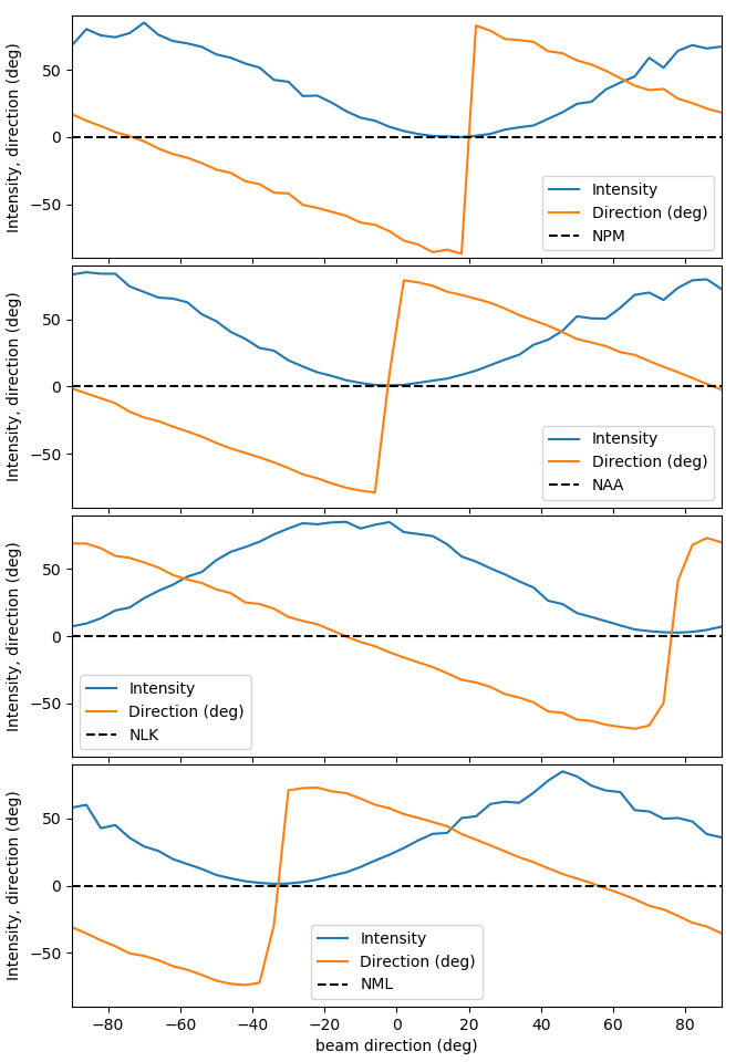
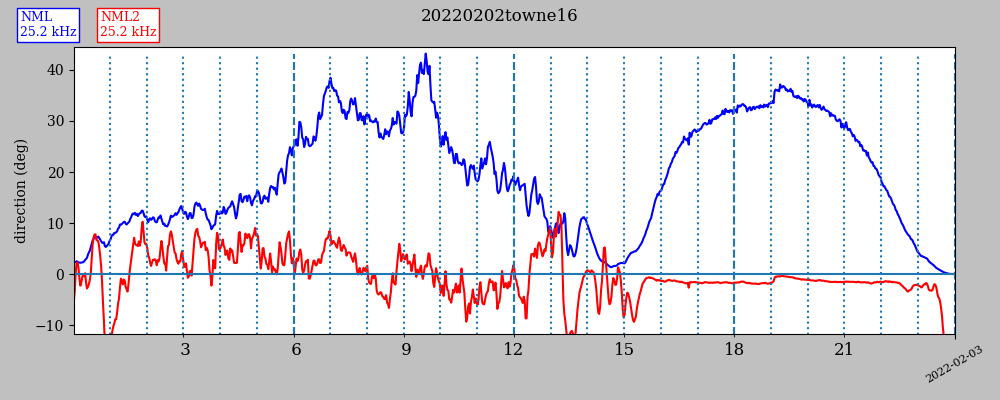
Each blue trace is of the intensity of its transmitter. The orange trace is of the angle of the transmitter relative to the primary beam direction, i.e., the pointing error. The legend entry for the dashed line (zero) is the transmitter name. We are looking for the pointing angle at which the intensity is greatest and the pointing error is zero, meaning where the primary beam is on the transmitter's bearing. For example, NML's zero crossing in the third graph is at -15°, and this value is entered in the transmitter's line in the header file. After taking data for one or more days, one can fine tune the beam angle using from a supersid_plot.py graph, such as shown in the following figure of NML direction (relative to its primary beam) during day-time hours where the signal is relatively stable.
src/supersid_plot.py -af <file path> -ps NMLd --vscale
During those hours, the transmitter direction is -0.5° from its primary beam. Although already small in this example, this difference can be set to zero for later data taking by shifting the beam angle in the transmitter line in the header file by 0.5°, the sign of which is determined by the slope in the scan figure above. Do not perform this step based on data taken during night-time hours as the signal direction, like the intensity, varies erratically during those turbulent hours.
Note that the slope of the error angle as a function of beam angle need not be negative. It depends on which of the antennae is channel 0. Also, because the loops can be flipped, which reverses the sign of the intercepted flux, this orientation of the loop affects the slope as well. So one may set the slope as part of the setup by reversing the channel assignments, reversing the leads of one of the loops, or flipping one of the antennae. This orientation also affects the sign of the angular error represented in the data.
One other antenna note. The antenna must be mounted securely. The direction noise level of the instrument can be as good as 0.1°, and at times even better. Any angular movement of one or both loops, e.g., by 1°, will spoil that low noise level. Even swaying or flexure of the wires in the wind on a larger spindle results in direction noise. So when delving into direction measurements with sidmon, additional care in the fabrication of the antenna is called for.
As was mentioned earlier, with two antennae sidmon coherently combines the two data streams for a primary beam pointed toward a transmitter, and an orthogonal beam perpendicular to it. In effect, sidmon computes x and y coordinates of the transmitter from those two synthesized beams, taking the arc tangent to get an angular direction. As with sidmon 2, there is fitting for intensity, but with sidmon 3 there is also fitting of the orthogonal beam, doubling the number of fits. So when plotting using live-plot sidmon.py -lp 2, there is a second column of plots showing the orthogonal fits and their qualities. An example is shown in the next plot.
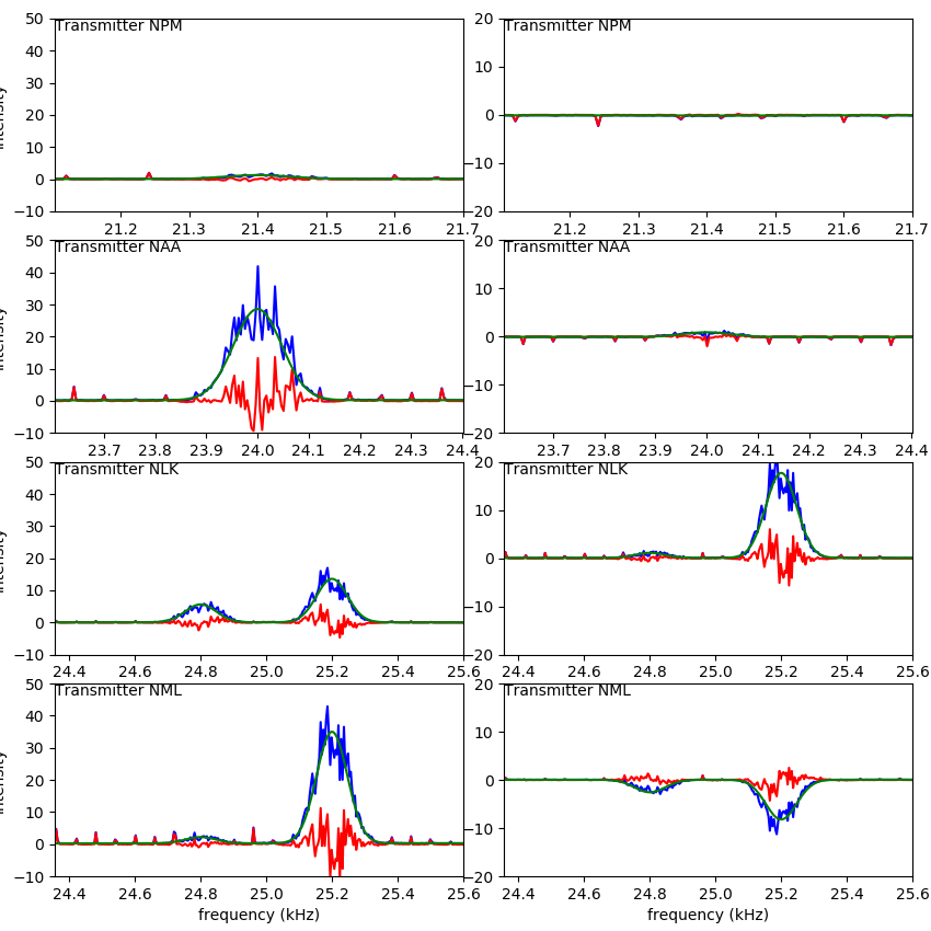
Notice in the second column that the intensities can be negative, representing signal bearing that are either left or right of the primary beam. Further interpretation of the those plots is nuanced due to groups containing more that one transmitter, necessary because closely spaced lines can overlap. Each transmitter has a row, and all transmitters in that transmitter's group are in the row and fitted. But only the fit of the transmitter of the row counts because the pointing is for the row's transmitter only. Thus the necessity of each transmitter having a row.
For example above, the third and fourth rows for NLK and NML are of the same group and are fitted together, but with NLK pointing in the third row, and NML pointing in the fourth.
git clone -b correlate --single-branch https://git.code.sf.net/p/sidmon3/code sidmonThis will create the directory sidmon. Note that without the switches, an older branch is incorrectly installed. The installation document provides a lot of detail for setting up a Raspberry Pi, and the install file will install several core dependencies from the internet when setting up a desktop computer.
Nathan Towne
towne56 at ownmail dot net
2/2022